Loss-Versus-Rebalancing Under Management

An empirical note on measuring loss-versus-rebalancing for an actively managed concentrated liquidity position. It assumes working familiarity with LVR and with concentrated liquidity positions on Uniswap v3 style automated market makers.

Two ways to read LVR

Loss-versus-rebalancing¹ is the cash loss of a liquidity position relative to a rebalancing strategy: a portfolio that holds the same token quantities as the position at every instant, trading at the external market price and paying no cost to do so. In the frictionless model it equals the profit of the arbitrageurs who keep the pool at that price. For a position that is simply passively left to its own devices, the loss depends on the price path only, and to leading order it is proportional to realised variance.²

A managed position however is not passive. When the price nears the edge of the range, the manager withdraws, re-centres and redeposits. Each re-centre mints a fresh position, and the proceeding loss accrues against that fresh position’s starting mix of tokens. The two common methods of putting a number to the loss of such a position do not agree.

Setup and notation

Stock estimate: the dashboard reading: the pool’s realised variance over the last 24 hours, applied to the range the position holds now and range-clipped, since outside that range the position’s token quantities are fixed. (“Stock” and “flow” are the operator’s names for its two bases; the literature would say trailing-window estimate.)

Realised loss: the exact reading: for each rebalance, what the position minted at the previous one lost against its own starting token quantities by the time it was replaced, summed over the day. In the literature’s terms, impermanent loss with the holdings benchmark updated at every rebalance, which is the rebalancing strategy loss with its benchmark reset at the operator’s own rebalance times.

$f$ : realised loss divided by stock estimate on a pool-day. $f = 1$ means the dashboard was right.

Rate: rebalances per pool per day.

Firing depth $\overline{∣ u ∣}$ : how far from the centre of the range the price had travelled when the manager fired, as a fraction of the half-width, averaged over the day: 0 is the centre, 1 the edge. (The firing position $u^{*}$ of the operator-fingerprinting paper,³ folded to the distance $d$ from the nearer edge, is $∣ u ∣ = 1 - 2 d$ .)

Flow estimate: a third reading, adopted by the operator in August 2026: the loss integrated as the price moves, on a five-minute clock.

The operator whose record this is ran on the stock estimate for seven months, using it as the loss side of its coverage ratio: emissions earned over loss-versus-rebalancing paid. In August 2026 it switched that ratio to the flow estimate. The comparison made at the switch, on seven weeks of data, found the stock estimate low by a factor of 2.57, and concluded that the gap could not be measured above about 150 rebalances a day. With the operation closed, the whole record can be read exactly.

The gap has been noticed before but as far as I can tell not measured. The 2026 revision of Milionis et al.¹ remarks that the empirical literature measures impermanent loss either against holdings fixed at a start date or as a sum over shorter intervals with the holdings benchmark updated, and that there is no theoretical guidance on which choice is correct. For a managed position, the difference between those two conventions is exactly $f$ , and the stock estimate uses the fixed-holdings one. On the practitioner side, a Bunni engineering note⁴ reports that tightly concentrated liquidity shifted quickly behind the price “locks in” its loss, and that its markouts, the value of its trades marked at a later price, are worse the faster it shifts. This is the same mechanism in the section below on why it is a rate law, seen from the trade side. The empirical studies of loss-versus-rebalancing on Uniswap v3⁵ measure passive positions, where the two conventions coincide.

The record

The operation managed concentrated liquidity on Aerodrome, the largest decentralised exchange on the Base network, from March to October 2026, rebalancing about a quarter of a million times across roughly 70 pools. Its own log kept the stock estimate at five-minute resolution, and from June it also recorded the previous range at every rebalance. Where both readings exist on a day with at least one rebalance there is a pool-day, of which there are about 1,450, on 30 pools. Each pool-day carries the rate, the width of the range in tick-spacings, and the firing depth.

Method, briefly

The exact reading uses the 107,869 rebalance intervals from June onwards, 99.6 per cent of which chain cleanly by position; the loss of each is computed from its two ticks and its range with the Uniswap v3 amount formulae, in units of the pair’s second token, and scaled by the position’s value at the later rebalance. Intervals over a week long or spanning more than 20,000 ticks are dropped as corrupt (474). The stock estimate is the daily median of the operator’s trailing-24-hour series. Confidence intervals are percentile bootstraps over pool-days, 2,000 draws. The code and the pool-day ratios will ship with the typeset note.

The ratio is a power of the rebalance rate

The figure is the whole result in one picture. Each dot is a pool-day. The higher the rebalance rate, the larger the ratio, and the relationship is a straight line on log axes.

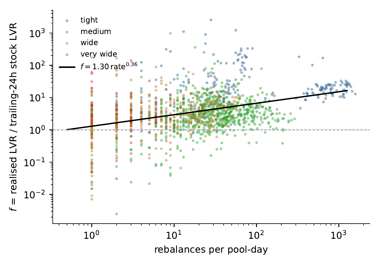
Realised-to-stock ratio f against rebalances per pool-day on 1,453 pool-days, coloured by the position's width class. The line is the fitted power law. The dashed line is f = 1, where the dashboard would have been right.

The fitted line is

lo g f = 0.26 + 0.356 lo g (rate), slope 95 % CI [0.31, 0.40] .

At one rebalance a day the stock estimate is low by about 30 per cent; at ten a day it shows a third of the loss; at a hundred a day, a seventh. The table gives the spread within each band; the last column is the same realised loss against the flow estimate, which exists from June.

Rebalances per pool-day	Pool-days	Median $f$	IQR	Median $f_{flow}$
< 5	287	2.0	0.9 – 4.3	3.2
5 – 20	394	2.6	1.4 – 6.0	2.0
20 – 50	455	4.0	2.1 – 7.7	2.2
50 – 150	213	4.8	2.5 – 8.9	2.4
≥ 150	104	14.1	8.2 – 22.0	2.2

Width class tells the same story in a different order, because width sets the rebalance rate: medium ranges 2.9, wide 2.6, very wide 2.9, tight 16.6. The three stable-pair pools with the narrowest ranges, one tick-spacing wide and fired between 38 and 1,067 times a day, read 16 to 21.

The understatement is not a constant that can be divided out; the 2.57 the operator measured at its August switch was simply the mix of rates its positions happened to run over those seven weeks. The stock estimate does not stop working above some rate; it just reads a smaller and smaller share of the loss smoothly all the way up.

The trigger enters twice

The rebalance rate is a consequence of the trigger rule, so changing the trigger changes $f$ . The question is whether it changes $f$ only by changing the rate, in which case every trigger sits on the same curve, or whether two triggers at the same rate can give different ratios.

Putting the trigger’s geometry into the fit answers it:

lo g f = - 0.40 + 0.356 lo g (rate) + 0.118 lo g (width / spacing) + 0.638 \overline{∣ u ∣} .

The confidence intervals are $[0.31, 0.40]$ on the rate, $[0.06, 0.18]$ on width and $[0.47, 0.93]$ on firing depth. The rate exponent is untouched by the extra terms. Firing depth is a second smaller channel. At the same rate, letting the price travel a further fifth of the half-width before firing raises $f$ by about 13 per cent. Width adds little once the rate is known.

The record also contains a natural experiment. On 30 July the trigger was changed on every position at once. The manager fires when the price comes within a fraction $φ$ of the range’s width of an edge; that fraction was randomised per range. And the centre of each new range, which must sit on the pool’s tick grid, had been rounded down by up to half a spacing; it was corrected to round to nearest. On the six pools held throughout, the rate fell from a median of 40 a day to 13. The rate law predicts the median $f$ falling from 4.0 to about 2.7; it fell to 2.2, about a sixth below. Firing depth did not move (0.65 to 0.67), so the shortfall is the part of the trigger that the second equation does not carry: placement and the randomisation of $φ$ . The curve shifted by about a quarter. Its slope did not change.

What the law is and is not

The one-variable form is written in the rate because the rate is the one number every operator can read straight off its own log. It is a reduced form: it holds for the trigger family that produced it, and another trigger sits on a curve shifted by a factor of the order of the depth and placement terms above, with the same exponent. This makes it more useful than a constant, because it says what to record in order to re-fit it: the rate and the mean firing position, per position, per day.

Why it is a rate law

The stock estimate takes the day’s variance and applies it to the range the position holds now. When the price leaves that range, the position’s token mixture is fully one sided, and the estimate stops accruing. For an unmanaged position this is correct, since a passive position does indeed stop losing once it is fully out of range.

A managed position is regularly brought back into range by being re-centred, which gives it a fresh exposure around the new centred price, and on the next price move it accrues loss again. The stock estimate, which only ever sees the current range, does not count what each earlier pre-rebalance range lost on that position’s closure. Each re-centring of a position is a loss the dashboard has already forgotten.

In symbols, the day’s realised loss is a sum over its $n$ rebalance intervals,

f = \frac{\sum _{i = 1}^{n} ℓ _{i}}{ℓ _{clip}},

where $ℓ_{i}$ is what the $i$ -th position lost between its mint and its replacement, and $ℓ_{clip}$ is the one clipped accrual the estimate reports for whichever range it happens to see. The numerator grows with $n$ , the rate, and with how much each position lost before it was reset, which is the firing depth. Both are trigger choices, and that is the whole content of the two-term fit. The exponent is below one because the two are not independent: at a higher rate each interval is shorter and each $ℓ_{i}$ smaller, so the ratio grows more slowly than the count.

The flow estimate integrates the loss as the price moves, so re-centring does not hide anything from it. The table shows it closing most of the gap and still reading about half the realised loss, flat in rate. What remains is a choice of clock: the exact reading resets its benchmark holdings at the operator’s rebalance times, the flow estimate every five minutes in this case, and the two agree only when both reset often.

The error of the cheap estimate is set by the manager’s own behaviour, and it is largest on exactly the positions that are managed hardest.

Consequences

Three follow, at the level of the measurement rather than of any strategy.

A coverage ratio built on the stock estimate overstates coverage by $f$ . Emissions over loss, fees over loss, any break-even that takes the stock estimate as its denominator, is too high by a factor that rises with how hard the position is churned. Any rule calibrated on it, whether to widen a range, to exit a pool or to enter one, is calibrated in units that move when the operator changes its trigger.

The correction is not a constant. The law has to be re-fitted on the operator’s own rebalance rate. The two things to record for that are the rebalance count and the firing depth, per position, per day; with those, the two-term fit can be refitted without the exact reading machinery.

For emission-funded positions, the bias points towards over-confidence. A position staked in a ve(3,3) gauge forfeits its swap fees and earns protocol emissions instead, an income that does not scale with price variance, so its break-even sits at a critical volatility.² An understated loss puts that critical volatility too high by a factor of $f^{1/2}$ , and by more on the pools that are churned most.

What this changes, and what it does not

The record is a single operator on one venue over seven months, with positions that forfeited swap fees in exchange for emissions and so carried the full loss without a fee offset. On a fee-earning position the exact reading would require a fee leg as well; the understatement in the loss leg is the same. The exponent is fitted onto rebalance rates from one to a thousand per day, and beyond that range it is an extrapolation. The rebalance firing-depth coefficient comes from one family of triggers and should be re-fitted before it is used on another.

None of the above changes the result. The dashboard’s error is not a constant, but it is set by the manager’s own behaviour and grows as a power of the rebalance rate.

References

J. Milionis, C. C. Moallemi, T. Roughgarden, A. L. Zhang. Automated Market Making and Loss-Versus-Rebalancing. arXiv:2208.06046 (2022; v6, May 2026). https://doi.org/10.48550/arXiv.2208.06046
Ryan, K. R. Loss-Versus-Rebalancing Under Emissions. Technical note (17 May 2026). lvr-under-emissions
Ryan, K. R. Operator Fingerprinting: Recovering and Defending the Hidden Rebalancing Policy of Concentrated Liquidity Managers. SSRN Preprint (2026). https://papers.ssrn.com/sol3/papers.cfm?abstract_id=7202340
Bunni. Dawn of LP Profitability. Engineering note. https://blog.bunni.xyz/posts/dawn-of-lp-profitability/
L. Heimbach, E. Schertenleib, R. Wattenhofer. Risks and Returns of Uniswap V3 Liquidity Providers. Proceedings of the 4th ACM Conference on Advances in Financial Technologies (2022). https://doi.org/10.48550/arXiv.2205.08904

gancor.xyz