Loss-Versus-Rebalancing Under Emissions

A technical note on loss-versus-rebalancing for emission-funded, gauge-staked ve(3,3) liquidity. This note is self-contained, but assumes working familiarity with LVR and concentrated liquidity AMMs.

The profitability condition

The loss-versus-rebalancing framework of Milionis, Moallemi, Roughgarden, and Zhang (2022)¹ gives a clean profitability condition for a passive AMM liquidity provider. The LP is ahead when cumulative fee income exceeds cumulative LVR, $F(T)>\mathrm{LVR}(T)$. Almost the entire LVR literature works on this condition, and therefore within the assumption that the LP collects the pool’s swap fees.

In emission-based DEXs, especially those in the ve(3,3) family, that assumption typically fails. A liquidity position staked in the emissions gauge does not ordinarily receive swap fees; those are redirected to vote-escrow holders, while the LP earns protocol emissions instead. The profitability condition therefore becomes $E(T)>\mathrm{LVR}(T)$, with $E$ the cumulative emission income.

This may appear to be a mere relabelling of the income term. It is not. Fee income and emission income have materially different dependence on volatility, and it is that difference which changes the regime.

A managed position has further terms, for instance gas, and in some architectures like the one I have recently written about, the per-rebalance dust redistribution, but the regime question turns only on $\mathrm{LVR}$ and the income term. The rest can therefore be set aside here.

Setup and notation

• LVR: loss-versus-rebalancing, the value an AMM liquidity provider loses against a benchmark that continuously rebalances to the AMM’s token composition at the true price and pays no arbitrage cost.
• $\sigma$: realised volatility of the pool’s log-price.
• Gauge-staking: in a ve(3,3) protocol (the Solidly lineage, Velodrome, Aerodrome, their Slipstream pools) a position staked in the pool’s gauge forfeits swap fees to vote-escrow holders and earns emissions of the native token instead.
• ${\epsilon }_P$: the gauge reward rate per unit of staked liquidity, set by veToken votes on a weekly epoch.
• $\psi (t)$: the in-range indicator, $1$ when the price sits inside the position’s range and $0$ otherwise; $\bar{\psi }$ is its time-average, the position’s time-in-range.
• em/LVR: cumulative emissions divided by cumulative LVR, the emission-side analogue of the fee-side break-even ratio.

LVR scales as ${\sigma }^2$

For a concentrated liquidity position with liquidity $L$ and price bounds $[P_a,P_b]$, while the position remains in range, the instantaneous LVR rate per dollar of position value is

$$\frac{d{\mathrm{LVR}}_{\$}}{dt}=\frac{{\sigma }^2}{4b},b=2-\sqrt{P_a/P}-\sqrt{P/P_b},$$

where $b$ is a bracket fixed by the range geometry and $P$ is the current price.

For a full-range position, $b$ tends to 2 and the rate reduces to the classical constant-product value ${\sigma }^2/8$. Out of range the rate is zero. The important point is that the LVR rate is proportional to ${\sigma }^2$. A more volatile price means quadratically more LVR.

Fee income also scales as ${\sigma }^2$

Fees are charged on swap volume. The volume that offsets LVR is arbitrage volume, that is, the trades which realign the pool with the market. Those same arbitrage trades are also what generate LVR. Fee income and LVR are therefore two read-outs of the same underlying process.²

Ovchinnikov, Khoudyakov, Skomorokhov, and Egorov (Curve, May 2026)³ made this precise for a fee-only constant-product pool. A proportional fee $f$ defines a no-arbitrage band of half-width $-\ln (1-f)$; arbitrage is then the reflection which keeps the AMM-market mispricing within that band. Writing $K$ for the cumulative reflection, fee revenue is retained as growth of the pool invariant,

$$\text{fee income}=\frac{f}{4-2f}K,\frac{\mathbb{E}[K]}{T}=\frac{{\sigma }^2}{2(-\ln (1-f))}.$$

Combining the two, and expanding $-\ln (1-f)=f+f^2/2+\dots$,

$$\frac{\text{fee income}}{T}=\frac{f}{4-2f}\cdot \frac{{\sigma }^2}{2(-\ln (1-f))}=\frac{{\sigma }^2}{8}+O(f^2{\sigma }^2),$$

which is exactly the constant-product LVR rate ${\sigma }^2/8$. Fee income therefore cancels LVR to first order in the fee, leaving an $O(f^2{\sigma }^2)$ residual.

The result is stated for the constant-product case, but the same local scaling carries over to a concentrated liquidity position while it remains in range. A V3 position is locally a constant-product LP with the same liquidity and the same instantaneous gamma, which is precisely the property used above to write its LVR rate as ${\sigma }^2/(4b)$. The common ${\sigma }^2$ factor is therefore local to the curve, not peculiar to the full-range case.

Accordingly, while the position is in range, fee income and LVR both accrue over the same interval, carry the same bracket $b$, and are gated by the same in-range fraction $\bar{\psi }$. Those common terms cancel in the ratio. The Monte Carlo below uses a range-clipped V3 position and confirms the point directly.

The point to carry forward is not the equality itself, but the volatility dependence. Fee income carries the same factor ${\sigma }^2$ as LVR, so $F/\mathrm{LVR}=2f/[(2-f)(-\ln (1-f))]=1+O(f^2)$, independent of $\sigma$. The fee-funded LP’s break-even is therefore flat in volatility, because numerator and denominator scale together.

Following the Skorokhod formulation, the fee-side picture here is the arbitrage-only limit. It counts the fees paid by arbitrageurs and sets aside organic, uninformed order flow.⁴ Organic fees track volume rather than ${\sigma }^2$, so a real fee-funded pool carries a roughly $\sigma$-flat income component on top of the arbitrage one. That introduces a mild ${\sigma }^{-2}$ term into a measured $F/\mathrm{LVR}$. It softens the contrast with the emission side without removing it. The fee-side break-even is $\sigma$-flat in its arbitrage core, and that core is the like-for-like comparison, because LVR is itself an arbitrage quantity.

Emission income does not scale with $\sigma$

The emission rate to a gauge-staked position is

$$\frac{dE}{dt}={\epsilon }_{P}L\psi (t)p_{\text{emission}}$$

with ${\epsilon }_P$ the gauge reward rate, $L$ the staked liquidity, and $p_{\text{emission}}$ the USD price of the emitted token. The term that matters is ${\epsilon }_P$. The reward rate is set by veToken votes on a weekly epoch, allocating the protocol’s inflation across gauges.

To leading order, ${\epsilon }_P$ is not a functional of the pool’s price process. A quiet pool may receive a large ${\epsilon }_P$ and a violent pool a small one, with a freedom no fee-funded income would permit.

There is, however, one qualification. The voters on a gauge receive the swap fees forfeited by the gauge’s staked LPs, alongside any bribes, so a rational voter has reason to favour high-fee, and hence high-volume, and often higher-$\sigma$ pools. Vote-set ${\epsilon }_P$ therefore inherits a weak and lagged dependence on volatility through the voters’ own fee income.

The incentive for a voter to favour high-fee pools is real, but the vote market acts on it loosely. A quantity of vote weight does not reprice to per-pool fee differentials, and instead votes via standing delegations or with votes carried forward, and the weekly epoch lags. Emission allocation ends up imperfectly tracking per-pool fee productivity. The leading-order picture, ${\epsilon }_P$ exogenous to $\sigma$, is the idealisation the rest of this note adopts, and the weak fee-coupling just described is the first correction to it.

So the emission-side numerator carries $\sigma$ only weakly, through a second-order channel, where the fee-side numerator carries it in full.

The ${\sigma }^{-2}$ regime

Form the break-even ratio. Evaluate the LVR rate at the position’s geometric-centre price, so that the bracket $b$ and the position value $V$ may be treated as constants over the window, and write both accruals explicitly:

$$E(T)={\epsilon }_{P}L{p}_{\text{emission}}{\int }_0^T\psi dt,\mathrm{LVR}(T)=\frac{V{\sigma }^2}{4b}{\int }_0^T\psi dt.$$

Emission accrual and LVR accrual are gated by the same indicator $\psi (t)$. The integral ${\int }_0^T\psi dt$ is therefore common to both, and cancels in the ratio:

$$\boxed{em/LVR=\frac{E(T)}{\mathrm{LVR}(T)}=\frac{4{\epsilon }_P{p}_{\text{emission}}Lb}{V{\sigma }^2}=\kappa {\sigma }^{-2}}$$

with $\kappa =4{\epsilon }_P{p}_{\text{emission}}Lb/V$. Since the in-range value of the position is $V=L\sqrt{P}b$, the staked liquidity $L$ and the bracket $b$ cancel, leaving $\kappa =4{\epsilon }_P{p}_{\text{emission}}/\sqrt{P}$. This is independent of $\sigma$, provided the emitted-token price is uncorrelated with the pool’s own volatility; a market-wide volatility spike, in which the two co-move, is the exception. Because $L$ and $b$ drop out, em/LVR is a property of the gauge and the pool, the same for every position in a given gauge whatever its size or range width.

The emission-funded break-even therefore scales as the inverse square of volatility. A fee-funded LP’s break-even is flat in $\sigma$. An emission-funded LP’s break-even falls as ${\sigma }^{-2}$. That is the regime distinction.

Why the in-range fraction does not spoil this

The time-in-range $\bar{\psi }=T^{-1}{\int }_0^T\psi dt$ is itself a decreasing function of $\sigma$. A more volatile price path leaves the range more often. So neither $E$ nor $\mathrm{LVR}$ is individually a clean power of $\sigma$; each carries $\bar{\psi }(\sigma )$. But $\bar{\psi }$ enters both as the same multiplicative gate, and therefore cancels in the ratio. The ${\sigma }^{-2}$ scaling is a property of the ratio, and it survives a volatility-dependent time-in-range. A marginal statement about either term on its own does not capture that.

Why there is no emission-side cancellation

The fee-side cancellation does not carry over to the emission case, not even in weakened form. The tempting assumption that some version of it must survive is wrong.

The cancellation rests on three features of fee income.

Feature of fee income	Holds for emissions?
It is a functional of the arbitrage reflection $K$	No. $E$ is paid by the gauge, not generated by $K$.
That reflection scales as ${\sigma }^2$	No. ${\epsilon }_P$ is vote-set, $\sigma$-independent.
One parameter $f$ fixes both the skim rate and the no-arbitrage band, pinning the prefactor to the LVR constant	No. ${\epsilon }_P$ and $\sigma$ are outputs of unrelated processes, and no common parameter links them.

Fee income and LVR are two read-outs of one process, namely arbitrage flow, and when two quantities are both proportional to the same underlying object, that object cancels in their ratio. Emission income is exogenous to that flow.

Set $f=0$, as gauge-staking does, and the band collapses, the reflection-driven income vanishes, and the income is supplied from outside the pool entirely. Each of the three features fails at the root. The fee-side cancellation, the dynamic-fee designs that tune it,⁵ and any analysis that treats the fee tier as the control variable all operate on income that co-moves with $\sigma$. None of them specialises to the emission case.

A spectrum

It is useful to order LP income by its volatility elasticity $\eta$, the exponent in income $\propto {\sigma }^{\eta }$. Since $\mathrm{LVR}\propto {\sigma }^2$, the break-even ratio scales as ${\sigma }^{\eta -2}$.

Income model	$\eta$	Break-even scaling	Cancellation
Static proportional fee	$2$	${\sigma }^0$	full first-order cancellation
Dynamic / adaptive fee	tunable	${\sigma }^{\eta -2}$	cancellation partially restored
Pure emission (gauge-staked)	$0$	${\sigma }^{-2}$	no cancellation

The fee literature sits at the first row, and has increasingly moved towards the second. The emission-funded position sits at the third, and that regime has not, to my knowledge, been cleanly described.

A Monte Carlo check

A controlled demonstration settles it more firmly than an assertion. A Monte Carlo is sufficient, and requires no real-world data.

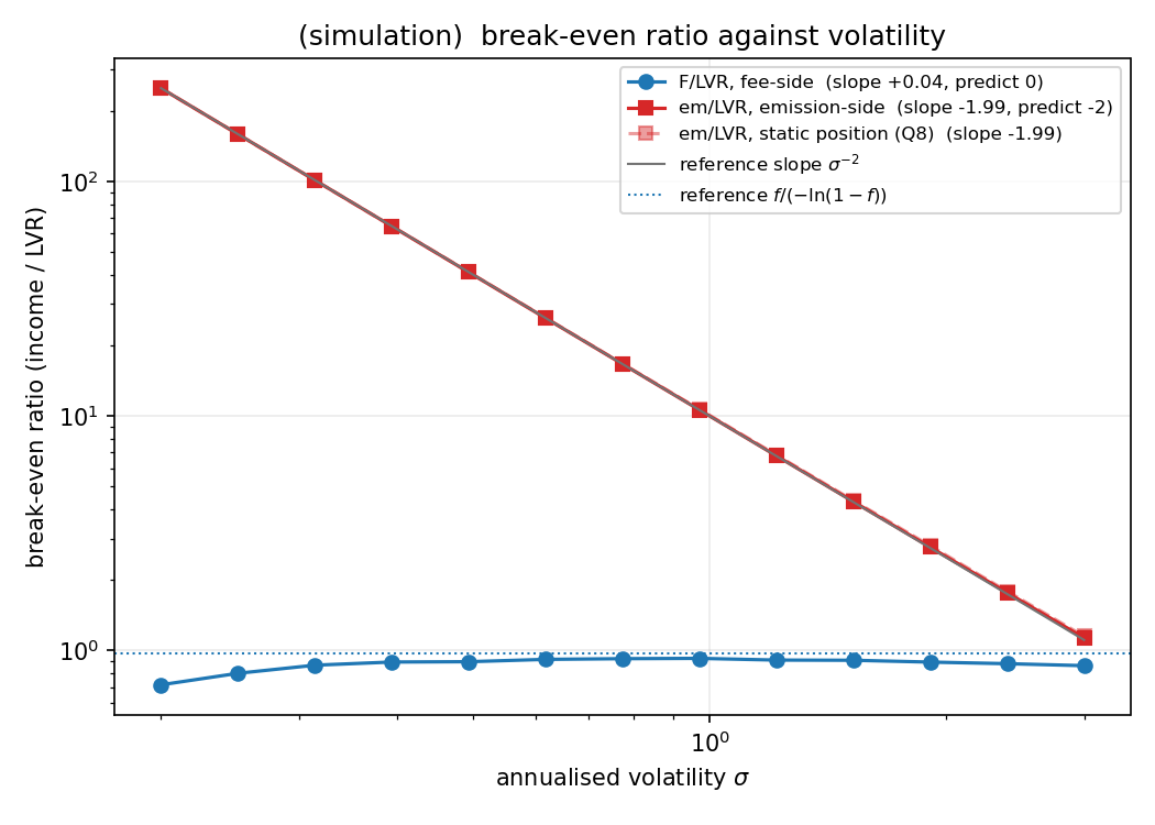
Take geometric Brownian price paths across a grid of volatilities, from 20 per cent to 300 per cent annualised. Run a representative concentrated liquidity position across each path. Accrue its LVR from the realised path by the range-clipped quadratic variation method, so that volatility enters only as the path parameter and no estimator is fed in. On the same paths accrue two income streams: a fee income, simulated as the band-reflected arbitrage throughput that a fee-collecting LP would skim, and an emission income at a fixed rate. The fee tier is set deliberately large so the no-arbitrage band is resolvable at a feasible time step; the simulation therefore demonstrates the volatility scaling of each quantity, the fitted slopes below, not the precise level of $F/\mathrm{LVR}$, which approaches one only as the fee tends to zero.

Fitted exponents

Log-log fits of quantity against $\sigma$, 13-point grid:

Quantity	Fitted slope	Predicted
LVR	$+1.99$	$+2$
Fee income	$+2.04$	$+2$
Emission income	$-0.00$	$0$
$F/\mathrm{LVR}$	$+0.04$	$0$
$em/LVR$	$-1.99$	$-2$

Holding the position un-recentred so its time-in-range falls from $0.98$ to $0.17$ across the grid leaves the $em/LVR$ fit unchanged at $-1.99$. The in-range fraction cancels in the ratio, exactly as it should.

Consequences

Three consequences follow, at the level of the framework rather than a strategy.

A definite critical volatility. Since $em/LVR=\kappa {\sigma }^{-2}$, the break-even $em/LVR=1$ is crossed at ${\sigma }_{\text{crit}}=\sqrt{\kappa }$. Every emission-funded pool has a volatility above which emissions no longer cover LVR. Because the scaling is a clean inverse square, ${\sigma }_{\text{crit}}$ is a definite property of the pool rather than a vague threshold. For a fee-funded LP there is no analogous critical volatility, because $F/\mathrm{LVR}$ is flat.

The right diagnostic is em/LVR, not em/IL. Operator dashboards in this space often report emissions over impermanent loss, with IL measured against simply holding the initial tokens. That benchmark is the wrong one. Impermanent loss against buy-and-hold is not the LVR cost; it mixes the cost with a rebalancing-convexity term, $V_{\text{REB}}-V_{\text{HODL}}$, the gap between the continuously-rebalanced and the buy-and-hold benchmarks, that has nothing to do with arbitrage.⁶ The LVR-consistent ratio is em/LVR, and it is that ratio which carries the ${\sigma }^{-2}$ structure.

LVR becomes an allocation question. Under fees, the LP is largely a price-taker on both sides of the break-even, with $\sigma$ exogenous and the fee tier fixed once the pool is chosen. Under emissions, the income side is a policy variable, ${\epsilon }_P$ is set by votes, and the choice of pool is itself an allocation problem. That shifts the question from measurement towards allocation. That is as far as this note takes the point.

When the allocation mechanism changes

The ${\sigma }^{-2}$ regime rests on one assumption: that emission income is, to leading order, exogenous to $\sigma$. As noted above, that is very nearly a property of vote-market allocation; the weak fee-coupling through voters’ fee income is the only qualification, and a vote market responds to a pool’s volatility only loosely and with a lag. Change the allocation mechanism so that the response becomes direct and fast, and the regime changes with it.

Aerodrome’s proposed V3 redesign, predictive allocation, is intended to do precisely that. The design is public so far only in draft specifications and an explanatory FAQ,⁷ rather than a final settlement specification, so the account here is necessarily provisional and may not match the mechanism that ultimately ships.

As presently drafted, the system replaces vote-directed emissions with a continuous allocation market. Stakers, formerly lockers (vote-escrow holders), direct emission weight to pools and receive the swap-fee revenue of the pools they allocate to. Because the reward for allocation is the pool’s fees, allocators have reason to favour fee-productive pools, and emissions are pulled towards tracking fee generation. The draft describes two further channels moving in the same direction; a global emission rate set as a multiple of protocol fees, and per-pool caps steered towards a fee-to-emissions target.

Fees co-move with $\sigma$. A fee-coupled allocation mechanism therefore tightens the coupling of ${\epsilon }_P$ to volatility, and on the spectrum above, moves the gauge-staked position off the $\eta =0$ pole towards the fee pole. The break-even correspondingly flattens from ${\sigma }^{-2}$ towards $\sigma$-flat. In that sense predictive allocation acts as a synthetic fee, engineering the co-movement that gauge-staking removed.

How tight that coupling becomes depends on parameters the published drafts treat as provisional. The channels as currently configured all respond slowly to volatility: the global rate is reset on a manual, daily-to-weekly cadence, the caps move at an operator’s discretion, and allocations sit under a 48-hour cooldown the team has described as an initial-phase setting it intends to tighten. If that holds, instantaneous ${\epsilon }_P$ stays exogenous to instantaneous $\sigma$, so the ${\sigma }^{-2}$ regime survives for the transient, high-frequency part of volatility and the flattening reaches only the persistent part the slow channels have had time to track; the break-even’s volatility exponent becomes a function of timescale. A faster or more direct coupling than the current drafts suggest would flatten more of the curve. The direction is the same either way; only the degree is uncertain.

This still leaves the regime claim falsifiable. The framework predicts that $em/LVR$ flattens on a protocol once it moves to fee-coupled allocation, and stays close to ${\sigma }^{-2}$ on one still running a vote market. The mechanism, not the token, is what places an emission-funded LP in the regime.

The shape of the gap

The canonical condition $F>\mathrm{LVR}$ was built for fee-collecting liquidity providers, and the literature refining it has remained within that assumption. A growing share of on-chain liquidity is gauge-staked and emission funded. For that liquidity, the condition becomes $E>\mathrm{LVR}$, with an income term largely exogenous to the volatility on which the loss depends. That single change in the source of income breaks the fee-side cancellation and places the break-even on a ${\sigma }^{-2}$ curve. It is a small observation with a definite shape, and it is the piece of the emission-funded picture the existing framework does not contain.

---

References

1. J. Milionis, C. C. Moallemi, T. Roughgarden, A. L. Zhang. Automated Market Making and Loss-Versus-Rebalancing. arXiv:2208.06046 (2022). https://doi.org/10.48550/arXiv.2208.06046
2. J. Milionis, C. C. Moallemi, T. Roughgarden. Automated Market Making and Arbitrage Profits in the Presence of Fees. In Financial Cryptography and Data Security (FC 2024), Lecture Notes in Computer Science 14744, Springer, Cham (2025). https://doi.org/10.1007/978-3-031-78676-1_9
3. G. V. Ovchinnikov, A. A. Khoudyakov, F. A. Skomorokhov, M. Egorov. Loss-versus-Rebalancing Cancellation in AMMs under Constant Volatility: A Reflected Skorokhod Equation Approach. Curve Letters (May 2026). https://github.com/curvefi/curve-letters
4. R. Fritsch, A. Canidio. Measuring Arbitrage Losses and Profitability of AMM Liquidity. Companion Proceedings of the ACM Web Conference 2024 (WWW ‘24), ACM, pp. 1761–1767. https://doi.org/10.1145/3589335.3651961
5. I. Lebedeva, D. Umnov, Y. Yanovich, I. Melnikov, G. Ovchinnikov. Dynamic Fee for Reducing Impermanent Loss in Decentralized Exchanges. IEEE International Conference on Blockchain and Cryptocurrency (ICBC) 2025. https://doi.org/10.1109/ICBC64466.2025.11114646
6. Á. Cartea, F. Drissi, M. Monga. Decentralized Finance and Automated Market Making: Predictable Loss and Optimal Liquidity Provision. SIAM Journal on Financial Mathematics 15(3), 931–959 (2024). https://doi.org/10.1137/23M1602103
7. Aero. Predictive Allocation FAQ. aero.xyz/articles/aero-predictive-allocation-faq (2026). Formal design drafts: Dromos Labs, MetaDEX specifications, github.com/dromos-labs/metadex-specs.